Introducing the WebKit FTL JIT
Just a decade ago, JavaScript – the programming language used to drive web page interactions – was thought to be too slow for serious application development. But thanks to continuous optimization efforts, it’s now possible to write sophisticated, high-performance applications – even graphics-intensive games – using portable standards-compliant JavaScript and HTML5. This post describes a new advancement in JavaScript optimization: the WebKit project has unified its existing JavaScript compilation infrastructure with the state-of-the-art LLVM optimizer. This will allow JavaScript programs to leverage sophisticated optimizations that were previously only available to native applications written in languages like C++ or Objective-C.
All major browser engines feature sophisticated JavaScript optimizations. In WebKit, we struck a balance between optimizations for the JavaScript applications that we see on the web today, and optimizations for the next generation of web content. Websites today serve large amounts of highly dynamic JavaScript code that typically runs for a relatively short time. The dominant cost in such code is the time spent loading it and the memory used to store it. These overheads are illustrated in JSBench, a benchmark directly based on existing web applications like Facebook and Twitter. WebKit has a history of performing very well on this benchmark.
WebKit also features a more advanced compiler that eliminates dynamic language overhead. This compiler benefits programs that are long-running, and where a large portion of the execution time is concentrated in a relatively small amount of code. Examples of such code include image filters, compression codecs, and gaming engines.
As we worked to improve WebKit’s optimizing compiler, we found that we were increasingly duplicating logic that would already be found in traditional ahead-of-time (AOT) compilers. Rather than continue replicating decades of compiler know-how, we instead investigated unifying WebKit’s compiler infrastructure with LLVM – an existing low-level compiler infrastructure. As of r167958, this project is no longer an investigation. I’m happy to report that our LLVM-based just-in-time (JIT) compiler, dubbed the FTL – short for Fourth Tier LLVM – has been enabled by default on the Mac and iOS ports.
This post summarizes the FTL engineering that was undertaken over the past year. It first reviews how WebKit’s JIT compilers worked prior to the FTL. Then it describes the FTL architecture along with how we solved some of the fundamental challenges of using LLVM as a dynamic language JIT. Finally, this post shows how the FTL enables a couple of JavaScript-specific optimizations.
Overview of the WebKit JavaScript Engine
This section outlines how WebKit’s JavaScript engine worked prior to the addition of the FTL JIT. If you are already familiar with concepts such as profile-directed type inference and tiered compilation, you can skip this section.
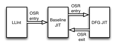
Prior to the FTL JIT, WebKit used a three-tier strategy for optimizing JavaScript, as shown in Figure 1. The runtime can pick from three execution engines, or tiers, on a per-function basis. Each tier takes our internal JavaScript bytecode as input and either interprets or compiles the bytecode with varying levels of optimization. Three tiers are available: the LLInt (Low Level Interpreter), Baseline JIT, and DFG JIT (Data Flow Graph JIT). The LLInt is optimized for low latency start-up, while the DFG is optimized for high throughput. The first execution of any function always starts in the interpreter tier. As soon as any statement in the function executes more than 100 times, or the function is called more than 6 times (whichever comes first), execution is diverted into code compiled by the Baseline JIT. This eliminates some of the interpreter’s overhead but lacks any serious compiler optimizations. Once any statement executes more than 1000 times in Baseline code, or the Baseline function is invoked more than 66 times, we divert execution again to the DFG JIT. Execution can be diverted at almost any statement boundary by using a technique called on-stack replacement, or OSR for short. OSR allows us to deconstruct the bytecode state at bytecode instruction boundaries regardless of the execution engine, and reconstructs it for any other engine to continue execution using that engine. As Figure 1 shows, we can use this to transition execution to higher tiers (OSR entry) or to deoptimize down to a lower tier (OSR exit; more on that below).
The three-tier strategy provides a good balance between low latency and high throughput. Running an optimizing JIT such as the DFG on every JavaScript function would be prohibitively expensive; it would be like having to compile an application from source each time you wanted to run it. Optimizing compilers take time to run and JavaScript optimizing JIT compilers are no exception. The multi-tier strategy ensures that the amount of CPU time – and memory – that we commit to optimizing a JavaScript function is always proportional to the amount of CPU time that this function has previously used. The only a priori assumption about web content that our engine makes is that past execution frequency of individual functions is a good predictor for those functions’ future execution frequency. The three tiers each bring unique benefits. Thanks to the LLInt, we don’t waste time compiling, and space storing, code that only runs once. This might be initialization code in a top-level <script> tag or some JSONP content that sneaked past our specialized JSON path. This conserves total execution time since compiling takes longer than interpreting if each statement only executes once; the JIT compiler itself would still have to loop and switch over all of the instructions in the bytecode, just as the interpreter would do. The LLInt’s advantage over a JIT starts to diminish as soon as any instruction executes more than once. For frequently executed code, about three quarters of the execution time in the LLInt is spent on indirect branches for dispatching to the next bytecode instruction. This is why we tier up to the Baseline JIT after just 6 function invocations or if a statement reexecutes 100 times: this JIT is responsible primarily for removing interpreter dispatch overhead, but otherwise the code that it generates closely resembles the code for the interpreter. This enables the Baseline JIT to generate code very rapidly, but it leaves some performance optimizations on the table, such as register allocation and type specialization. We leave the advanced optimizations to the DFG JIT, which is invoked only after the code reexecutes in the Baseline JIT enough times.
The DFG JIT converts bytecode into a more optimizable form that attempts to reveal the data flow relationships between operations; the details of the DFG’s intermediate code representation are closest to the classic continuation-passing style (CPS) form that is often used in compilers for functional languages. The DFG does a combination of traditional compiler optimizations such as register allocation, control flow graph simplification, common subexpression elimination, dead code elimination, and sparse conditional constant propagation. But serious compilers require knowledge about the types of variables, and the structures of objects in the heap, to perform optimizations. Hence the DFG JIT uses profiling feedback from the LLInt and Baseline JIT to build predictions about the types of variables. This allows the DFG to construct a guess about the type of any incoming value. Consider the following simple program as an example:
function foo(a, b) { return a + b + 42; }
Looking at the source code alone, it is impossible to tell if a and b are numbers, strings, or objects; and if they are numbers, we cannot tell if they will be integers or doubles. Hence we have the LLInt and Baseline JIT collect value profiles for each variable whose value originates in something non-obvious, like a function parameter or load from the heap. The DFG won’t compile foo until it has executed lots of times, and each execution will contribute values to the profiles of these parameters. For example, if the parameters are integers, then the DFG will be able to compile this function with cheap ‘are you an integer?’ checks for both parameters, and overflow checks on the two additions. No paths for doubles, string concatenation, or calls to object methods like valueOf() will need to be generated, which saves both space and total execution time. If these checks fail, the DFG will use on-stack replacement (OSR) to transfer execution back to the Baseline JIT. In this way, the Baseline JIT serves as a permanent fall-back for whenever any of the DFG’s speculative optimizations are found to be invalid.
An additional form of profiling feedback are the Baseline JIT’s polymorphic inline caches. Polymorphic inline caches are a classic technique for optimizing dynamic dispatch that originated in the Smalltalk community. Consider the following JavaScript function:
function foo(o) { return o.f + o.g; }
In this example, the property accesses may lead to anything from a simple load from well-known locations in the heap to invocations of getters or even complicated DOM traps, like if o were a document object and “f” were the name of an element in the page. The Baseline JIT will initially execute these property accesses as fully polymorphic dispatch. But as it does so it will record the steps it takes, and will then modify the heap accesses in-place to be caches of the necessary steps to repeat a similar access in the future. For example, if the object has a property “f” at offset 16 from the base of the object, then the code will be modified to first quickly check if the incoming object consists of a property “f” at offset 16 and then perform the load. These caches are said to be inline because they are represented entirely as generated machine code. They are said to be polymorphic because if different object structures are encountered, the machine code is modified to switch on the previously encountered object types before doing a fully dynamic property lookup. When the DFG compiles this code, it will check if the inline cache is monomorphic – optimized for just one object structure – and if so, it will emit just a check for that object structure followed by the direct load. In this example, if o was always an object with properties “f” and “g” at invariant offsets, then the DFG would only need to emit one type check for o followed by two direct loads.
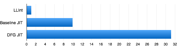
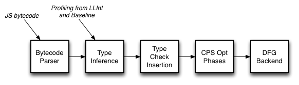
Figure 2 shows an overview of the DFG optimization pipeline. The DFG uses value profiles and inline caches as a starting point for type inference. This allows it to generate code that is specialized just for the types that we had previously observed. The DFG then inserts a minimal set of type checks to guard against the program using different types in the future. When these checks fail, the DFG will OSR exit back to Baseline JIT’s code. Since any failing check causes control to leave DFG code, the DFG compiler can optimize the code following the check under the assumption that the check does not need to be repeated. This enables the DFG to aggressively minimize the set of type checks. Most reuses of a variable will not need any checks.
Figure 3 shows the relative speed-up of each of the tiers on one representative benchmark, an OS simulation by Martin Richards. Each tier takes longer to generate code than the tiers below it, but the increase in throughput due to each tier more than makes up for it.
The three-tier strategy allows WebKit to adapt to the requirements and characteristics of JavaScript code. We choose the tier based on the amount of time the code is expected to spend running. We use the lower tiers to generate profiling information that serves to bootstrap type inference in the DFG JIT. This works well – but even with three tiers, we are forced to make trade-offs. We frequently found that tuning the DFG JIT to do more aggressive optimizations would improve performance on long-running code but would hurt short-running programs where the DFG’s compile time played a larger role in total run-time than the quality of the code that the DFG generated. This led us to believe that we should add a fourth tier.
Architecting a Fourth Tier JIT
WebKit’s strengths arise from its ability to dynamically adapt to different JavaScript workloads. But this adaptability is only as powerful as the tiers that we have to choose from. The DFG couldn’t simultaneously be a low-latency optimizing compiler and a compiler that produced high-throughput code – any attempts to make the DFG produce better code would slow it down, and would increase latency for shorter-running code. Adding a fourth tier and using it for the heavier optimizations while keeping the DFG relatively light-weight allows us to balance the requirements of longer- and shorter-running code.
The FTL JIT is designed to bring aggressive C-like optimizations to JavaScript. We wanted to ensure that the work we put into the FTL impacted the largest variety of JavaScript programs – not just ones written in restricted subsets – so we reused our existing type inference engine from the DFG JIT and our existing OSR exit and inline cache infrastructure for dealing with dynamic types. But we also wanted the most aggressive and comprehensive low-level compiler optimizations. For this reason, we chose the Low Level Virtual Machine (LLVM) as our compiler backend. LLVM has a sophisticated production-quality optimization pipeline that features many of the things we knew we wanted, such as global value numbering, a mature instruction selector, and a sophisticated register allocator.
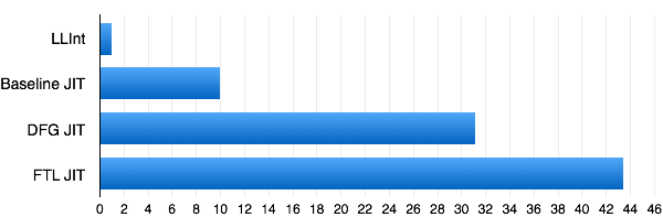
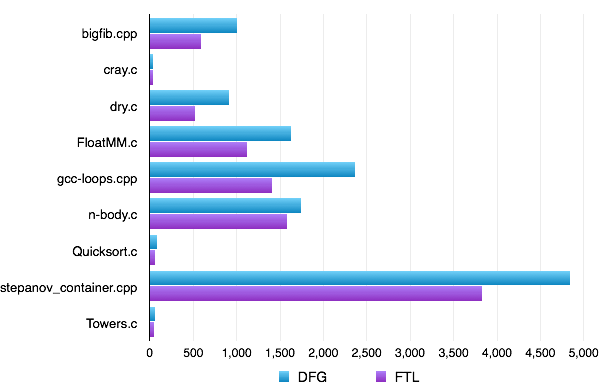
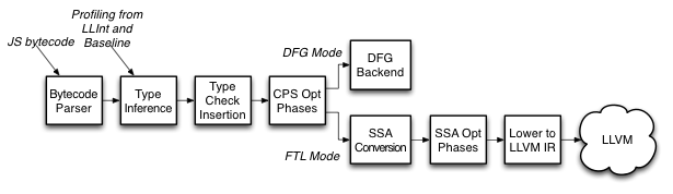
Figure 4 shows an overview of the FTL architecture. The FTL exists primarily in the form of an alternate backend for the DFG. Instead of invoking the DFG’s machine code generator – which is very fast but does almost no low-level optimizations – we convert the DFG’s representation of the JavaScript function into static single assignment (SSA) form and perform additional optimizations. Conversion to SSA is more expensive than the DFG’s original CPS conversion but it enables more powerful optimizations, like loop-invariant code motion. Once those optimizations are done, we convert the code from the DFG SSA form to LLVM IR. Since LLVM IR is also based on SSA, this is a straight-forward linear and one-to-many conversion. It only requires one pass over the code, and each instruction within the DFG SSA form results in one or more LLVM IR instructions. At this point, we eliminate any JavaScript-specific knowledge from the code. All JavaScript idioms are lowered to either an inlined implementation of the JavaScript idiom using LLVM IR, or a procedure call if we know that the code path is uncommon.
This architecture gives us freedom to add heavy-weight optimizations to the FTL while retaining the old DFG compiler as a third tier. We even have the ability to add new optimizations that work within both the DFG and FTL by adding them before the “fork” in the compilation pipeline. It also integrates well with the design of the LLVM IR: LLVM IR is statically typed, so we need to perform our dynamic language optimizations before we transition to LLVM IR. Fortunately, the DFG is already good at inferring types – so by the time that LLVM sees the code, we will have ascribed types to all variables. Converting JavaScript to LLVM IR turns out to be quite natural with our indirect approach – first the source code turns into WebKit’s bytecode, then into DFG CPS IR, then DFG SSA IR, and only then into LLVM IR. Each transformation is responsible for removing some of JavaScript’s dynamism and by the time we get to LLVM IR we will have eliminated all of it. This allows us to leverage LLVM’s optimization capabilities even for ordinary human-written JavaScript; for example on the Richards benchmark from Figure 3, the FTL provides us with an additional 40% performance boost over the DFG as shown in Figure 5. Figure 6 shows a summary of what the FTL gives us on asm.js benchmarks. Note that the FTL isn’t special-casing for asm.js by recognizing the "use asm" pragma. All of the performance is from the DFG’s type inference and LLVM’s low-level optimizing power.
The WebKit FTL JIT is the first major project to use the LLVM JIT infrastructure for profile-directed compilation of a dynamic language. To make this work, we needed to make some big changes – in WebKit and LLVM. LLVM needs significantly more time to compile code compared to our existing JITs. WebKit uses a sophisticated generational garbage collector, but LLVM does not support intrusive GC algorithms. Profile-driven compilation implies that we might invoke an optimizing compiler while the function is running and we may want to transfer the function’s execution into optimized code in the middle of a loop; to our knowledge the FTL is the first compiler to do on-stack-replacement for hot-loop transfer into LLVM-compiled code. Finally, LLVM previously had no support for the self-modifying code and deoptimization tricks that we rely on to handle dynamic code. These issues are described in detail below.
Side-stepping LLVM Compile Times
Compiler design is subject to a classic latency-throughput trade-off. It’s hard to design a compiler that can generate excellent code quickly – the compilers that generate code most rapidly also generate the worst code, while compilers like LLVM that generate excellent code are usually slow. Moreover, where a compiler lands in the latency-throughput continuum tends to be systemic; it’s hard to make a compiler that can morph from low-latency to high-throughput or vice-versa.
For example, the DFG’s backend generates mediocre code really quickly. It’s fast at generating code precisely because it does just a single pass over a relatively high-level representation; but this same feature means that it leaves lots of optimization opportunities unexploited. LLVM is the opposite. To maximize the number of optimization opportunities, LLVM operates over very low-level code that has the best chance of revealing redundancies and inefficient idioms. In the process of converting that code to machine code, LLVM performs multiple lowering transformations through several stages that involve different representations. Each representation reveals different opportunities for speed-ups. But this also means that there is no way to short-circuit LLVM’s slowness compared to the DFG. Just converting code to LLVM’s IR is more costly than running the entire DFG backend, because LLVM IR is so low-level. Such is the trade-off: compiler architects must choose a priori whether their compiler will have low latency or high throughput.
The FTL project is all about combining the benefits of high-throughput and low-latency compilation. For short running code, we ensure that we don’t pay the price of invoking LLVM unless it’s warranted by execution count profiling. For long-running code, we hide the cost of invoking LLVM by using a combination of concurrency and parallelism.
Our second and third tiers – the Baseline and DFG JITs – are invoked only when the function gets sufficiently “hot”. The FTL is no different. No function will be compiled by the FTL unless it has already been compiled by the DFG. The DFG then reuses the execution count profiling scheme from the Baseline JIT. Each loop back-edge adds 1 to an internal per-function counter. Returning adds 15 to the same counter. If the counter crosses zero, we trigger compilation. The counter starts out as a negative value that corresponds to an estimate of the number of “executions” of a function we desire before triggering a higher-tier compiler. For Baseline-to-DFG tier-up, we set the counter to -1000 × C where C is a function of the size of the compilation unit and the amount of available executable memory. C is usually close to 1. DFG-to-FTL tier-up is more aggressive; we set the counter to -100000 × C. This ensures that short-running code never results in an expensive LLVM-based compile. Any function that runs for more than approximately 10 milliseconds on modern hardware will get compiled by the FTL.
In addition to a conservative compilation policy, we minimize the FTL’s impact on start-up time by using concurrent and parallel compilation. The DFG has been a concurrent compiler for almost a year now. Every part of the DFG’s pipeline is run concurrently, including the bytecode parsing and profiling. With the FTL, we take this to the next level: we launch multiple FTL compiler threads and the LLVM portion of the FTL’s pipeline can even run concurrently to WebKit’s garbage collector. We also keep a dedicated DFG compiler thread that runs at a higher priority, ensuring that even if we have FTL compilations in the queue, any newly discovered DFG compilation opportunities take higher priority.
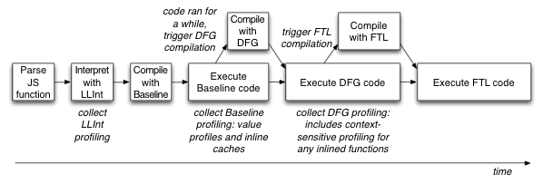
Figure 7 illustrates the timeline of a function as it tiers-up from the LLInt all the way to the FTL. Parsing and Baseline JIT compilation are still not concurrent. Once Baseline JIT code starts running, the main thread will never wait for the function to be compiled since all subsequent compilation happens concurrently. Also, the function will not get compiled by the DFG, much less the FTL, if it doesn’t run frequently enough.
Integrating LLVM with Garbage Collection
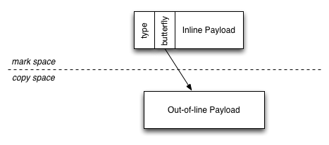
WebKit uses a generational garbage collector with a non-moving space for object cells, which hold fixed-size data, and a hybrid mark-region/copy space for variable-size data (see Figure 8). The generation of objects is tracked by a sticky mark bit. Our collector also features additional optimizations such as parallel collection and carefully tuned allocation and barrier fast paths.
Our approach to integrating garbage collection with LLVM is designed to maximize throughput and collector precision while eliminating the need for LLVM to know anything about our garbage collector. The approach that we use, due to Joel Bartlett, has been known since the late 1980’s and we have already been using it for years. We believe, for high-performance systems like WebKit, that this approach is preferable to a fully conservative collector like Boehm-Demers-Weiser or various accurate collection strategies based on forcing variables to be spilled onto the stack. Full Boehm-style conservatism means that every pointer-sized word in the heap and on the stack is conservatively considered to possibly be a pointer. This is both slow – each word needs to be put through a pointer testing algorithm – and very imprecise, risking retention of lots of dead objects. On the other hand, forcing anything – pointers or values suspected to be pointers – onto the stack will result in slow-downs due to additional instructions to store those values to memory. One of our reasons for using LLVM is to get better register allocation; placing things on the stack goes against this goal. Fortunately, Bartlett garbage collection provides an elegant middle ground that still allows us to use a sophisticated generational copying collector.
In a Bartlett collector, objects in the heap are expected to have type maps that tell us which of their fields have pointers and how those pointers should be decoded. Objects that are only reachable from other heap objects may be moved and pointers to them may be updated. But the stack is not required to have a stack map and objects thought to be referenced from the stack must be pinned. The collector’s stack scan must: (1) ensure that it reads all registers in addition to the stack itself, (2) conservatively consider every pointer-width word to possibly be a pointer, and (3) pin any object that looks like it might be reachable from the stack. This means that the compilers we use to compile JavaScript are allowed to do anything they want with values and they do not have to know whether those values are pointers or not.
Because program stacks are ordinarily several orders of magnitude smaller than the rest of the heap, the likelihood of rogue values on the stack accidentally causing a large number of dead heap objects to be retained is very low. In fact, over 99% of objects in a typical heap are only referenced from other heap objects, which allows a Bartlett collector to move those objects – either for improved cache locality or to defragment the heap – just as a fully accurate collector would. Retention of some dead objects is of course possible, and we can tolerate it so long as it corresponds to only a small amount of space overhead. In practice, we’ve found that so long as we use additional stack sanitization tricks – such as ensuring that our compilers use compacted stack frames and occasionally zeroing regions of the stack that are known to be unused – the amount of dead retention is negligible and not worth worrying about.
We had initially opted to go with the Bartlett approach to garbage collection because it allowed our runtime to be written in ordinary C++ that directly referenced garbage collected objects in local variables. This is both more efficient – no overhead from object handles – and easier to maintain. The fact that this approach also allowed us to adopt LLVM as a compiler backend without requiring us to handicap our performance with stack spilling has only reinforced our confidence in this well-known algorithm.
Hot-loop Transfer
One of the challenges of using multiple execution engines for running JavaScript code is replacing code compiled by one compiler with code compiled by another, such as when we decide to tier-up from the DFG to the FTL. This is usually easy. Most functions have a short lifecycle – they will tend to return shortly after they are called. This is true even in the case of functions that account for a large fraction of total execution time. Such functions tend to be called frequently rather than running for a long time during a single invocation. Hence our primary mechanism for replacing code is to edit the data structures used for virtual call resolution. Additionally, for any calls that were devirtualized, we unlink all incoming calls to the function’s old code and then relinking them to the newly compiled code. For most functions this is enough: shortly after the newly optimized code is available, all previous calls into the function return and all future calls go into optimized code.
While this is effective for most functions, sometimes a function will run for a long time without returning. This happens most frequently in benchmarks – particularly microbenchmarks. But sometimes it affects real code as well. One example that we found was a typed array initialization loop, which runs 10× faster in the FTL than in the DFG, and the difference is so large that its total run-time in the DFG is significantly greater than the time it takes to compile the function with the FTL. For such functions, it makes sense to transfer execution from DFG-compiled code to FTL-compiled code while the function is running. This problem is called hot-loop transfer (since this will only happen if the function has a loop) and in WebKit’s code we refer to this as OSR entry.
It’s worth noting that LLInt-to-Baseline and Baseline-to-DFG tier-up already supports OSR entry. OSR entry into the Baseline JIT takes advantage of the fact that we trivially know how the Baseline JIT represents all variables at every instruction boundary. In fact, its representation is identical to the LLInt, so LLInt-to-Baseline OSR entry just involves jumping to the appropriate machine code address. OSR entry into the DFG JIT is slightly more complicated since the DFG JIT will typically represent state differently than the Baseline JIT. So the DFG makes OSR entry possible by treating the control flow graph of a function as if it had multiple entrypoints: one entrypoint for the start of the function, and one entrypoint at every loop header. OSR entry into the DFG operates much like a special function call. This inhibits many optimizations but it makes OSR entry very cheap.
Unfortunately the FTL JIT cannot use either approach. We want LLVM to have maximum freedom in how it represents state and there doesn’t exist any mechanism for asking LLVM how it represents state at arbitrary loop headers. This means we cannot do the Baseline style of OSR entry. Also, LLVM assumes that functions have a single entrypoint and changing this would require significant architectural changes. So we cannot do the DFG style of OSR entry, either. But more fundamentally, having LLVM assume that execution may enter a function through any path other than the function’s start would make some optimizations – like loop-invariant code motion, or LICM for short – harder. We want the FTL JIT to be able to move code out of loops. If the loop has two entrypoints – one along a path from the function’s start and another via OSR entry – then LICM would have to duplicate any code it moves out of loops, and hoist it into both possible entrypoints. This would represent a significant architectural challenge and would, in practice, mean that adding new optimizations to the FTL would be more challenging than adding those optimizations in a compiler that can make the single-entrypoint assumption. In short, the complexity of multiple entrypoints combined with the fact that LLVM currently doesn’t support it means that we’d prefer not to use such an approach in the FTL.
The approach we ended up using for hot-loop transfer is to have a separate copy of a function for each entrypoint that we want to use. When a function gets hot enough to warrant FTL compilation, we opportunistically assume that the function will eventually return and reenter the FTL by being called again. But, if the DFG version of the function continues to get hot after we already have an FTL compilation and we detect that it is getting hot because of execution counting in a loop, then we assume that it would be most profitable to enter through that loop. We then trigger a second compile of that function in a special mode called FTLForOSREntry, where we use the loop pre-header as the function’s entrypoint. This involves a transformation over DFG IR where we create a new starting block for the function and have that block load all of the state at the loop from a global scratch buffer. We then have the block jump into the loop. All of the code that previously preceded the loop ends up being dead. Thus, from LLVM’s standpoint, the function takes no arguments. Our runtime’s OSR entry machinery then has the DFG dump its state at the loop header into that global scratch buffer and then we “call” the LLVM-compiled function, which will load the state from that scratch buffer and continue execution.
FTL OSR entry may involve invoking LLVM multiple times, but we only let this happen in cases where we have strong evidence to suggest that the function absolutely needs it. The approach that we take requires zero new features from LLVM and it maximizes the optimization opportunities available to the FTL.
Deoptimization and Inline Caches
Self-modifying code is a cornerstone of high-performance virtual machine design. It arises in three scenarios that we want our optimizing JavaScript compilers to be able to handle:
Partial compilation. It’s common for us to leave some parts of a function uncompiled. The most obvious benefit is saving memory and compile times. This comes into play when using speculative optimizations that involve type checks. In the DFG, each operation in the original JavaScript code usually results in at least one speculative check – either to validate some value’s type or to ensure that some condition, like an array index being in-bounds, is known to hold. In some carefully written JavaScript programs, or in programs generated by a transpiler like Emscripten, it’s common for the majority of these checks to be optimized out. But in plain human-written JavaScript code many of these checks will remain and having these checks is still better than not performing any speculative optimizations. Therefore it’s important for the FTL to be able to handle code that may have thousands of “side exit” paths that trigger OSR to the Baseline JIT. Having LLVM compile these paths eagerly wouldn’t make sense. Instead, we want to patch these paths in lazily by using self-modifying code.
Invalidation. The DFG optimization pipeline is capable of installing watchpoints on objects in the heap and various aspects of the runtime’s state. For example, objects that are used as prototypes may be watchpointed so that any accesses to instances of the prototype can constant-fold the prototype’s entries. We also use this technique for inferring which variables are constants and this makes it easy for developers to use JavaScript variables the same way that they would use static final variables in Java. When these watchpoints fire – for example because an inferred-constant variable is written to ‐ we invalidate any optimized code that had made assumptions about those variables’ values. Invalidation means unlinking any calls to those functions and making sure that any callsites within the function immediately trigger OSR exit after their callees return. Both invalidation and the partial compilation are broadly part of our deoptimization strategy.
Polymorphic inline caches. The FTL has many different strategies for generating code for a heap access or function call. Both of these JavaScript operations may be polymorphic. They may operate over objects of many types, and the set of types that flow into the operation may be infinite – in JavaScript it is possible to create new objects or functions programmatically and our type inference may ascribe a different type to each object if a common type cannot be inferred. Most heap accesses and calls end up with a finite (and small) set of types that flow into it, and so the FTL can usually emit relatively straight-forward code. But our profiling may tell us that the set of types that flow into an operation is large. In that case, we have found that the best way of handling the operation is with an inline cache, just like what the Baseline JIT would do. Inline caches are a kind of dynamic devirtualization where the code we emit for the operation may be repatched as the types that the operation uses change.
Each of these scenarios can be thought of as self-modifying inline assembly, but at a lower level with a programmatic interface to patch the machine code contents and select which registers or stack locations should be used. Much like inline assembly, the actual content is decided by the client of LLVM rather than by LLVM itself. We refer to this new capability as a patchpoint and it is exposed in LLVM as the llvm.experimental.patchpoint intrinsic. The workflow of using the intrinsic looks as follows:
- WebKit (or any LLVM client) decides which values need to be available to the patchpoint and chooses the constraints on those values’ representation. It’s possible to specify that the values could be given in any form, in which case they may end up as compile-time constants, registers, register with addend (the value is recoverable by taking some register and adding a constant value to it), or memory locations (the value is recoverable by loading from the address computed by taking some register and adding a constant to it). It’s also possible to specify more fine-grained constraints by having the values passed by calling convention, and then selecting the calling convention. One of the available calling conventions is
anyreg, which is a very lightweight constraint – the values are always made available in registers but LLVM can choose which registers are used.WebKit must also choose the size, in bytes, of the machine code snippet, along with the return type.
-
LLVM emits a nop sled – a sequence of nop instructions – whose length is the size that WebKit chose. Using a separate data section that LLVM hands over to WebKit, LLVM describes where the nop sled appears in the code along with the locations that WebKit can use to find all of the arguments that were passed to the patchpoint. Locations may be constants, registers with addends, or memory locations.
LLVM also reports which registers are definitely in use at each patchpoint. WebKit is allowed to use any of the unused registers without worrying about saving their values.
-
WebKit emits whatever machine code it wants within the nop sleds for each patchpoint. WebKit may later repatch that machine code in whatever way it wants.
In addition to patchpoints, we have a more constrained intrinsic called llvm.experimental.stackmap. This intrinsic is useful as an optimization for deoptimization. It serves as a guarantee to LLVM that we will only overwrite the nop sled with an unconditional jump out to external code. Either the stackmap is not patched, in which case it does nothing, or it is patched in which case execution will not fall through to the instructions after the stackmap. This could allow LLVM to optimize away the nop sled entirely. If WebKit overwrites the stackmap, it will be overwriting the machine code that comes immediately after the point where the stackmap would have been. We envision the “no fall-through” rule having other potential uses as we continue to work with the LLVM project to refine the stackmap intrinsic.
Armed with patchpoints and stackmaps, the FTL can use all of the self-modifying code tricks that the DFG and Baseline JITs already use for dealing with fully polymorphic code. This guarantees that tiering-up from the DFG to the FTL is never a slow-down.
FTL Specific High-Level Optimizations
So far this post has given details on how we integrated with LLVM and managed to leverage its low-level optimization capabilities without losing the capabilities of our DFG JIT. But adding a higher-tier JIT also empowers us to do optimizations that would have been impossible if our tiering strategy ended with the DFG. The sections that follow show two capabilities that a fourth tier makes possible, that aren’t specific to LLVM.
Polyvariant Devirtualization
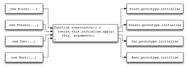
constructor at the new Point(...) callsite causes the call to initialize to always call Point’s initialize method.To understand the power of polyvariance, let’s just consider the following common idiom for creating classes in JavaScript:
var Class = {
    create: function() {
        function constructor() {
            this.initialize.apply(this, arguments);
        }
        return constructor;
    }
}
Frameworks such as Prototype use a more sophisticated form of this idiom. It allows the creation of class-like objects by saying Class.create(). The returned “class” can then be used as a constructor. For example:
var Point = Class.create();
Point.prototype = {
    initialize: function(x, y) {
        this.x = x;
        this.y = y;
    }
};
var p = new Point(1, 2); // Creates a new object p such that p.x == 1, p.y == 2
Every object instantiated with this idiom will involve a call to constructor, and the constructor’s use of this.initialize will appear to be polymorphic. It may invoke the Point class’s initialize method, or it may invoke the initialize methods of any of the other classes created this idiom. Figure 9 illustrates this problem. The call to initialize appears polymorphic, thereby preventing us from completely inlining the body of Point’s constructor at the point where we call new Point(1, 2). The DFG will succeed in inlining the body of constructor(), but it will stop there. It will use a virtual call for invoking this.initialize.
But consider what would happen if we then asked the DFG to profile its virtual calls in the same way that the Baseline JIT does. In that case, the DFG would be able to report that if constructor is inlined into an expression that says new Point(), then the call to this.initialize always calls Point.prototype.initialize. We call this polyvariant profiling and it’s one of the reasons why we retain the DFG JIT even though the FTL JIT is more powerful – the DFG JIT acts as a polyvariant profiler by running profiling after inlining. This means that the FTL JIT doesn’t just do more traditional compiler optimizations than the DFG. It also sees a richer profile of the JavaScript code, which allows it to do more devirtualization and inlining.
It’s worth noting that having two different compiler tiers, like DFG and FTL, is not strictly necessary for getting polyvariant profiling. For example, we could have eliminated the DFG compiler entirely and just had the FTL “tier up” to itself after gathering additional profiling. We could even have infinite recompilation with the same optimizing compiler, with any polymorphic idioms compiled with profiling instrumentation. As soon as that instrumentation observed opportunities for any additional optimizations, we could compile the code again. This could work, but it relies on polymorphic code always having profiling in case it might eventually be found to be monomorphic after all. Profiling can be very cheap – such as in the case of an inline cache – but there is no such thing as a free lunch. The next section shows the benefits of aggressively “locking in” all of the paths of a polymorphic access and allowing LLVM to treat it as ordinary code. This is why we prefer to use an approach where after some number of executions, a function will no longer have profiling for any of its code paths and we use a low-latency optimizing compiler (the DFG) as the “last chance” for profiling.
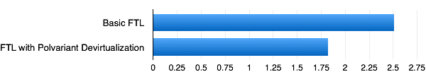
Figure 10 shows one of the benchmark speed-ups we get from polyvariant devirtualization. This benchmark uses the Prototype-style class system and does many calls to constructors that are trivially inlineable if we can devirtualize through the constructor helper. Polyvariant devirtualization is a 38% speed-up on this benchmark.
Polymorphic Inlining
The DFG has two strategies for optimizing heap accesses. Either the access is known to be completely monomorphic in which case the code for the access is inlined, or the access is turned into the same kind of inline cache that the Baseline JIT would have used. Inlined accesses are profitable because DFG IR can explicitly represent all of the steps needed for the access, such as the type checking, the loads of any intermediate pointers such as the butterfly (see Figure 8), any GC barriers, and finally the load or store. But if the access is believed to be polymorphic based on the available profiling, it’s better for the DFG to use an inline cache, for two reasons:
- The access may have been thought to be polymorphic but may actually end up being monomorphic. An inline cache can be very fast if the access ends up being monomorphic, perhaps because of imprecise profiling. As the previous section noted, the DFG sometimes sees imprecise profiling because the Baseline JIT knows nothing of calling context.
- The FTL wants to have additional profiling for polymorphic accesses in order to perform polyvariant devirtualization. Polymorphic inline caches are a natural form of profiling – we lazily emit only the code that we know we need for the types we know we saw, and so enumerating over the set of seen types is as simple as looking at what cases the inline cache ended up emitting. If we inlined the polymorphic access, we would lose this information, and so polyvariant profiling would be more difficult.
For these reasons, the DFG represents polymorphic operations – even ones where the number of incoming types is believed to be small and finite – as inline caches. But the FTL can inline the polymorphic operations just fine. In fact, doing so leads to some interesting optimization opportunities in LLVM.
We represent polymorphic heap accesses as single instructions in DFG IR. These instructions carry meta-data that summarizes all of the possible things that may happen if that instruction executes, but the actual control and data flow of the polymorphic operation is not revealed. This allows the DFG to cheaply perform “macro” optimizations on polymorphic heap accesses. For example, a polymorphic heap load is known to the DFG to be pure and so may be hoisted out of loops without any need to reason about its constituent control flow. But when we lower DFG IR to LLVM IR, we represent the polymorphic heap accesses as a switch over the predicted types and a basic block for each type. LLVM can then do optimizations on this switch. It can employ one of its many techniques for efficiently emitting code for switches. If we do multiple accesses on the same object in a row, LLVM’s control flow simplification can thread the control flow and eliminate redundant switches. More often, LLVM will find common code in the different switch cases. Consider an access like o.f where we know that o either has type T and “f” is at offset 24 or it has type U and “f” is at offset 32. We have seen LLVM be clever enough where it turns the access into something like:
o + 24 + ((o->type == U) < < 3)
In other words, what our compiler would have thought of as control flow, LLVM can convert to data flow, leading to faster and simpler code.
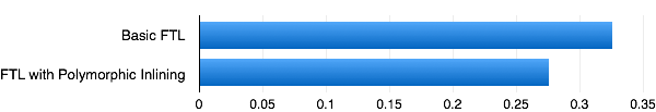
One of the benchmarks that benefited from our polymorphic inlining was Deltablue, shown in Figure 11. This program performs many heap accesses on objects with different structures. Revealing the nature of this polymorphism and the specific code paths for all of the different access modes on each field allows LLVM to perform additional optimizations, leading to a 18% speed-up.
Conclusion
Unifying the compiler infrastructures of WebKit and LLVM has been an extraordinary ride, and we are excited to finally enable the FTL in WebKit trunk as of r167958. In many ways, work on the FTL is just beginning – we still need to increase the set of JavaScript operations that the FTL can compile and we still have unexplored performance opportunities. In a future post I will show more details on the FTL’s implementation along with open opportunities for improvement. For now, feel free to try it out yourself in a WebKit nightly. And, as always, be sure to file bugs!